implied volatility is a price
May 03, 2023
new york
Why do we need an options pricing model?
In 1973, Black and Scholes published The Pricing of Options and Corporate Liabilities, inventing the Black-Scholes Options Pricing Model. One critical element of their model is that the value of an option with the price \(S\), strike \(K\), and maturity \(T\), is dependent on the variance of the underlying stock price.
This makes intuitive sense, the value of a call option is, at some level, a probability-weighted value, based on all possible futures values of the underlying stock price, minus the strike. If the price of the stock is highly volatile, it follows that there is a higher probability that the stock price will end up above the strike price, and therefore valuable to the owner of the option.
Importantly, the payoff distribution of options is asymmetric, that is the value of the option cannot be negative, but has unlimited upside. If the payoff was symmetric, a risk-neutral actor would be indifferent to the volatility of the stock price, because the distribution of upside gains is exactly matched by downside losses. This type of derivative is called a forward.
If we then look at the volatility of the stock and the asymmetric distribution of profits, we can see the value of an option. I have all the upside and none of the downside. Great! But how can I put a dollar value on the price of an option? One simple way would be, the price at which I can buy or sell it on the open market. But what if I don’t want to sell my option? Or what if I can’t find someone to sell me the option I want? Can I look at sales of other, similar options and estimate the value of mine based on those prices?
It’s not quite that simple, however. For example, let’s take a deep in-the-money option, say \(S = 100\), \(K = 50\), and \(T = 1\) month, and we believe that this stock price is not very volatile. The value of this option is very close to 50 (\(S - K\)), because the volatility is going to be equally distributed on the upside and downside, and the probability it ends up less than \(K\) in the next month is essentially 0%. So lets say that this option is worth 50. Compare that with an option where \(K = 52\). We are currently out-of-the-money (i.e., if we were to have the execute this option today, it’s value would be 0), but the probability that our stock price ends above 52 is not 0%. Within the market, we see options trading with the same T trading with strikes of 50, 55, and 65, but not 52. We observe that the prices for these options are not zero and we know that our option is more valuable than the options with strikes of 55 and 65, but also less valuable than the option with a strike of 50.
| Stock Price | Expiry | Strike Price | Value |
|---|---|---|---|
| 50 | 1 month | 50 | 2.92 |
| 50 | 1 month | 52 | ? |
| 50 | 1 month | 55 | 1.68 |
| 50 | 1 month | 60 | 1.12 |
| 50 | 1 month | 65 | 0.85 |
Perhaps we could take a weighted average approach: if the \(K = 50\) option is worth 2.92 and the \(K = 55\) option is worth 1.68, we can interpolate for our price and arrive at 2.424 (0.248 per unit of strike). However, if this methodology were to hold, we would expect the \(K = 65\) option to be worthless, but we can see willing buyers at 0.85. However, as we mentioned previously, the value of the option is a probability-weighted value, so as long as there is some probability that the price of the stock is above 65 in 5 days, there must be some value to that option. For that, we have Black-Scholes.
What is the Black-Scholes Model?
What Black and Scholes discovered is that you can think of an option as having two components. (1) An asset-or-nothing call and (2) a cash-or-nothing call. If we own the option, if the stock price is above the strike, we receive the asset (i.e., we own the asset-or-nothing call) and we pay the cash (i.e., we are are short the cash-or-nothing call).
(2) is fairly simple to understand, its value is the probability of the stock price being above the strike, multiplied by whatever the cash amount is that we’ll have to pay.
(1) is less obvious. Roughly, one can think of it as the moneyness of the stock price, expressed in standard deviations, multiplied by the stock price.
Leaving aside discounting, the value of a call option, using the Black-Scholes formula, can be expressed
$$ \begin{align} C &= SN(d_1) - KN(d_2) \\ d_1 &= \frac{1}{\sigma \sqrt{T}}\bigg[\ln \bigg(\frac{F}{K} \bigg) + \frac{1}{2} \sigma^2 T \bigg] \\ d_2 &= d_1 - \sigma \sqrt{T} \end{align} $$
Note that \(F\) is the forward price of the stock (i.e., the price you would have to pay for the stock if you agreed to buy it today, but we wouldn’t do the transaction until some defined future date).
To understand the implied volatility, you needn’t understand the minutae of the model, but note that sigma (\(\sigma\)) is the only variable we’ve not yet defined. That is the implied volatility.
What is implied volatility?
Now that we have the we know what an options model is and have a basic understanding of the Black-Scholes model, we can start to understand implied volatility. Implied volatility is the volatility implied by the option price. Put another way, if we know the price of an option (because it’s traded in the market), and we know the stock price and interest rates and all the other terms, we can simply solve for the implied volatility.
But why would we do that?
Simple – remember the problem we had above? How can I figure out the value of my \(K = 52\) option? Well, as we saw above, it wasn’t so straightforward to find out what the value of my option was despite what the fact that I know the values of other, very similar options that were both more and less valuable than mine. However, if I can figure out the implied volatility of those other options, perhaps I can use that to find the implied volatility of my option and then the price!
| Stock Price | Expiry | Strike Price | Value | Implied Volatility |
|---|---|---|---|---|
| 50 | 1 month | 50 | 2.92 | 50% |
| 50 | 1 month | 52 | ? | ? |
| 50 | 1 month | 55 | 1.68 | 60% |
| 50 | 1 month | 60 | 1.12 | 70% |
| 50 | 1 month | 65 | 0.85 | 80% |
And there we have it, the implied volatility of my option must be somewhere in between 50% - 60%. If we the apply our linear interpolation, we find that our implied volatility is 54%, and based on the Black-Scholes model, our option is worth 2.30! It makes sense, its a bit less than half-way between 2.92 and 1.68.
So, implied volatility is just the volatility implied by options prices. Is it anything else?
Certainly people in financial markets take it as a proxy for the expected volatility of a particular stock price. However, there is an historic pattern that observed volatility undershoots implied volatility. This makes sense, implied volatility is forward-looking, its risky. Just because volatility usually is below this level doesn’t mean that it always will be. If I’m going to take a risk and sell you this option, I need to make sure I’m getting paid for it.
Why is the implied volatility different for different strikes?
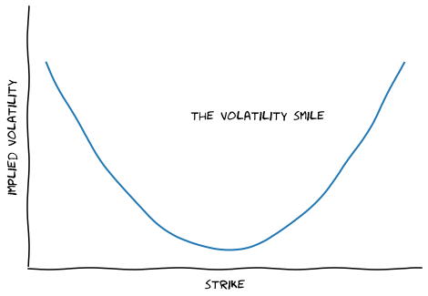
This is a particularly hard-to-answer question. This is an emergent phenomenon of volatility models. The further out-of-the-money you go, the higher the implied volatility. It’s called the volatility smile (since a plot looks like a U-shaped curve).
There’s no “right” answer to this question, but conventional wisdom is that the further out you go, the more you have to pay to encourage someone to sell you the option. If you’re buying that \(K = 65\) option, where the stock needs to go up by more than 30% in a single month to even start making money for the buyer, an option seller might logically think something’s up. And, as a result, she’s going to make you pay a bit more than if you were buy something that didn’t need such a large move. Of course, the actual price of the \(K = 55\) option is more expensive, but its cheaper in vol.
In a sense, for options, what you’re paying for is volatility1. And implied volatility is just a different representation of that price.
-
I am indebted to @Quantian1 for a series of tweets he wrote on this topic. ↩︎